Test Signals

🎯 Learning Objectives

By the end of this topic, you should be able to:

Let us start with some of the prerequisites required to progress through the topic. These are going to be simple enough in the first part of the contents. We will look at some of the test signals we will use to analyze the behavior of the filters. In the reset of session we will take a look at some of the basic building blocks that all filters need.
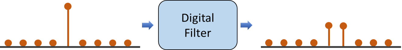
The idea here is to have a set of test signals that you can pass as an input to our theoretical filter and then observe the processed signal that we get out of the output. The key here is that this process should be deterministic and repeatable meaning no matter how many times we pass the input signal through the filter. We would need to get the same output regardless. Since we are in the digital domain and talking about digital filters, the input signals are merely just a set of numbers.
What do we want from our test signals? Well they need to be simple signals they don not necessarily have to be audio signals, just signals that are simple, concise and perhaps periodic. Since we are testing the frequency response of filters it helps to choose test signals that are well spread out across the Band frequencies.

Step Signal:

The first test signal is a DC signal or a 0 Hz signal as show in the Figure below.

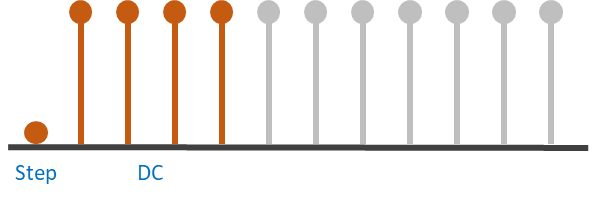
It starts at zero and steps up to 1. This signal contains two parts.

• The step portion where the input changes from 0 to 1 and
• The DC portion where the signal remains at a constant level of 1 forever

Because it stays at the same level there is no periodicity and thus its frequency said to be 0 Hz.
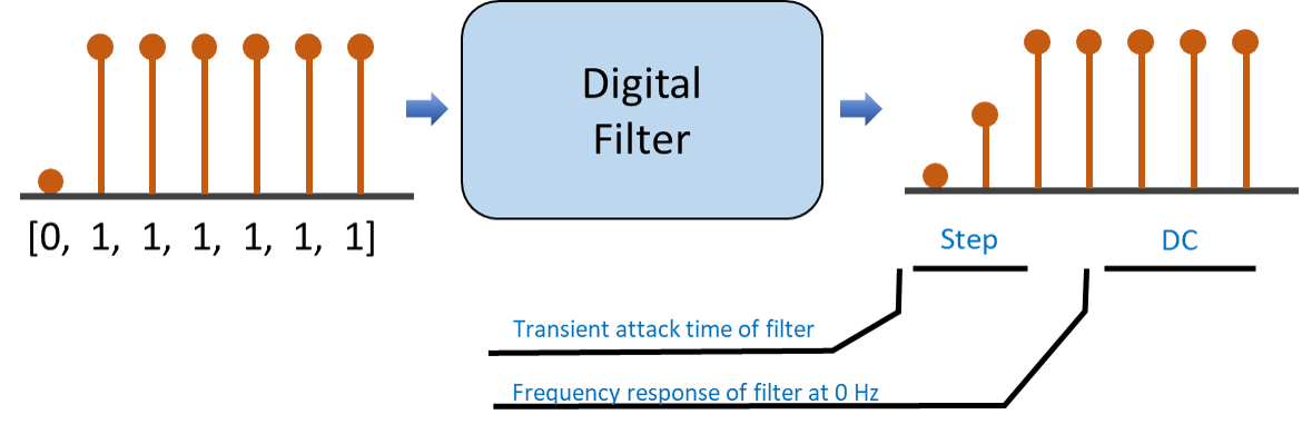
When we apply the signal to our DSP filter and examine the output we will get two pieces of information (as show in the Figure below)

• The step portion will tell us the transient attack time and
• The DC portion will give us the frequency response of the filter at 0 Hz.

This is illustrated in the following Figure

Periodic Signals:

Half Naquist Signal

The next test signal is a periodic signal at the Nyquist frequency. Simply, the Nyquist frequency is half the sampling rate. So if a system has a sample rate of 48 kHz, the Nyquist frequency is 24 kHz. This is the highest representable frequency for that sampling rate. We cannot represent frequencies higher than the Nyquist frequency for a given sample rate. For our test signal the Nyquist input sequence represents the Nyquist frequency of the system and is independent of the actual sampling rate. We don not care what the sample rate of the system is but we know that at the Nyquist frequency each cycle of a sinusoid can be represented by at most two data points. So, the input sequence of this test signal will be something as show in the Figure below, with each sample representing the maximum and minimum values of a cycle of a sinusoid.

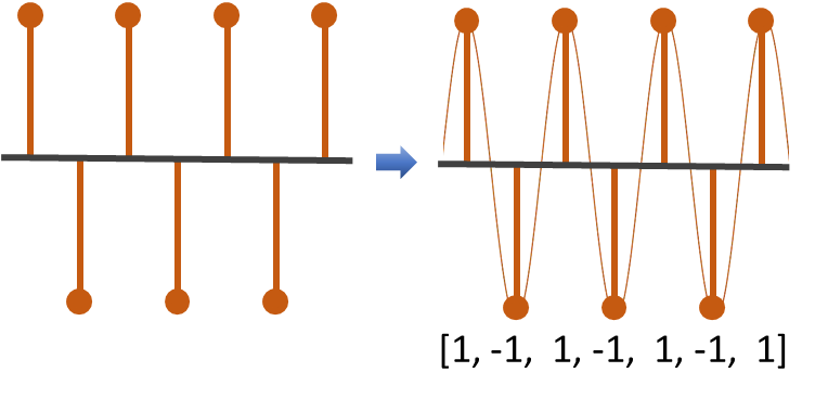
Note here that for the first single we chose 0 Hz, with is the minimum representable frequency and after that the Nyquist frequency signal which is the the maximum representable frequency.
So what we are doing here is selecting signals to test the boundary conditions of possible frequencies that a filter might encounter.

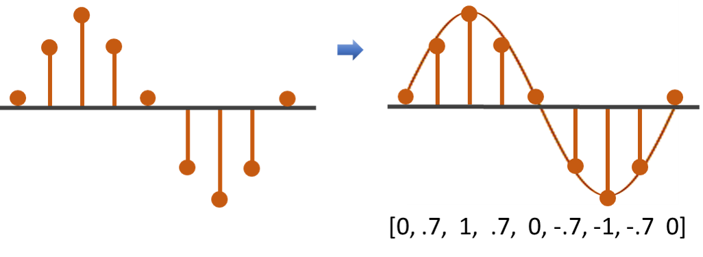
Quater Naquist Signal

For this frequency the signal is encoded with four samples per cycle twice as many as the Nyquist signal. For this frequency the signal is encoded with eight samples per cycle four times as many as the Nyquist signal and the sequence as show in Figure below. You can include several test signals of different frequencies if you need a wider range of inputs like 1/8 or 1/16 of a Nyquist but this is fine for now.

Impulse Signal

The impulse signal is a special case and it is quite important to describe the system. An Impulse signal is made up of a single sample value of one in an infinitely long stream of zeros as the name suggests. It is a singular impulse a tiny flick of an input. If we take this input signal and pass it through a DSP filter the output of the algorithm is called the impulse response. This is illustrated in the Figure below.

The terminology makes sense. It is the filter's response to an impulse. The impulse response of a digital algorithm characterizes the behavior of the system. The reason why the impulse response is so important and useful is that by knowing how a filter or an algorithm behaves to a unit impulse, we can calculate how it behaves to any arbitrary input. This is because any input signal can be thought of as being made up of a series of impulses or an Impulse train. If an input signal is just a series of impulses of different magnitude then we can use convolution to convolve the input signal and the impulse response signal to generate the output response for that signal.

Notions:

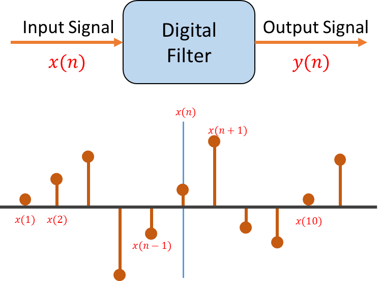
The input signal is termed as $x(n)$, where $n$ represents the location of the nth sample of the input sequence. Similarly the output signal is termed as $y(n)$. If we want to refer to individual samples we could do so as $x(1)$ or $x(2)$ or $x(10)$. But referring to absolute positioning of sample values gets cumbersome. Moreover, algorithms do not use the sample's absolute position in their coding, instead the algorithms use the position of the current input sample as their reference frame and make everything relative to that sample. So for this reason we use n as the current position of the input sample. So $x(n)$ is the current sample $x(n−1)$ would be the previous sample $x(n+1)$ will be the next sample in the sequence, a future sample. In this way, the frame of reference is always going to be the current sample and everything revolves around how the filter processes $x(n)$.

Algorithm Building Block:

Finally in this topic we will take a look at some of the simple DSP structures that form the basic building blocks of all DSP algorithms. So we will discuss them briefly here and use them in the next DSP topics. Here are some general representation of the these fundamental blocks.

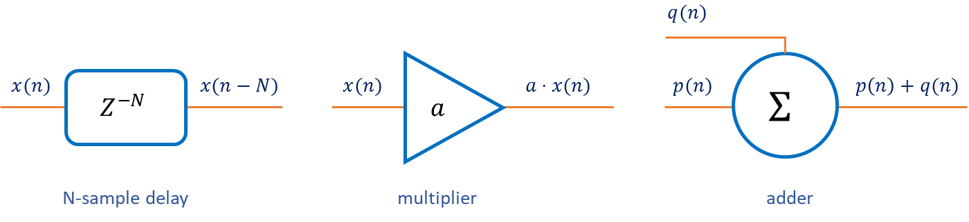
Lets understand them with examples. We will be talking about a simple one sample delay, a scalar multiplier and an adder.

Sample Delay:

So time delays are at the core of every digital filter. In our block diagram we can think about a delay structure or an algorithm as a black box labeled $Z$. The $Z$ term also has an exponent associated with it which signifies how many samples a signal is delayed by the exponent is a whole number like $Z^{−1}$, which signifies a one sample delay backwards in time. So if a signal $x(n)$ we were to go through a one sample delay block, the output would be the same sample delayed by exactly one sample and the signal is noted as $x(n−1)$. The exponent can be any arbitrary number like $Z^{−5}$, where the delay is 5 samples backwards or $Z^{0}$ which signifies no delay at all or $Z^{+1}$ which represents a delay forward in time to a future sample. This is a strange notation that how could you have a positive delay towards the future. The answer is that you cannot. The Figure below show the examples of what we discussed in above paragraph.

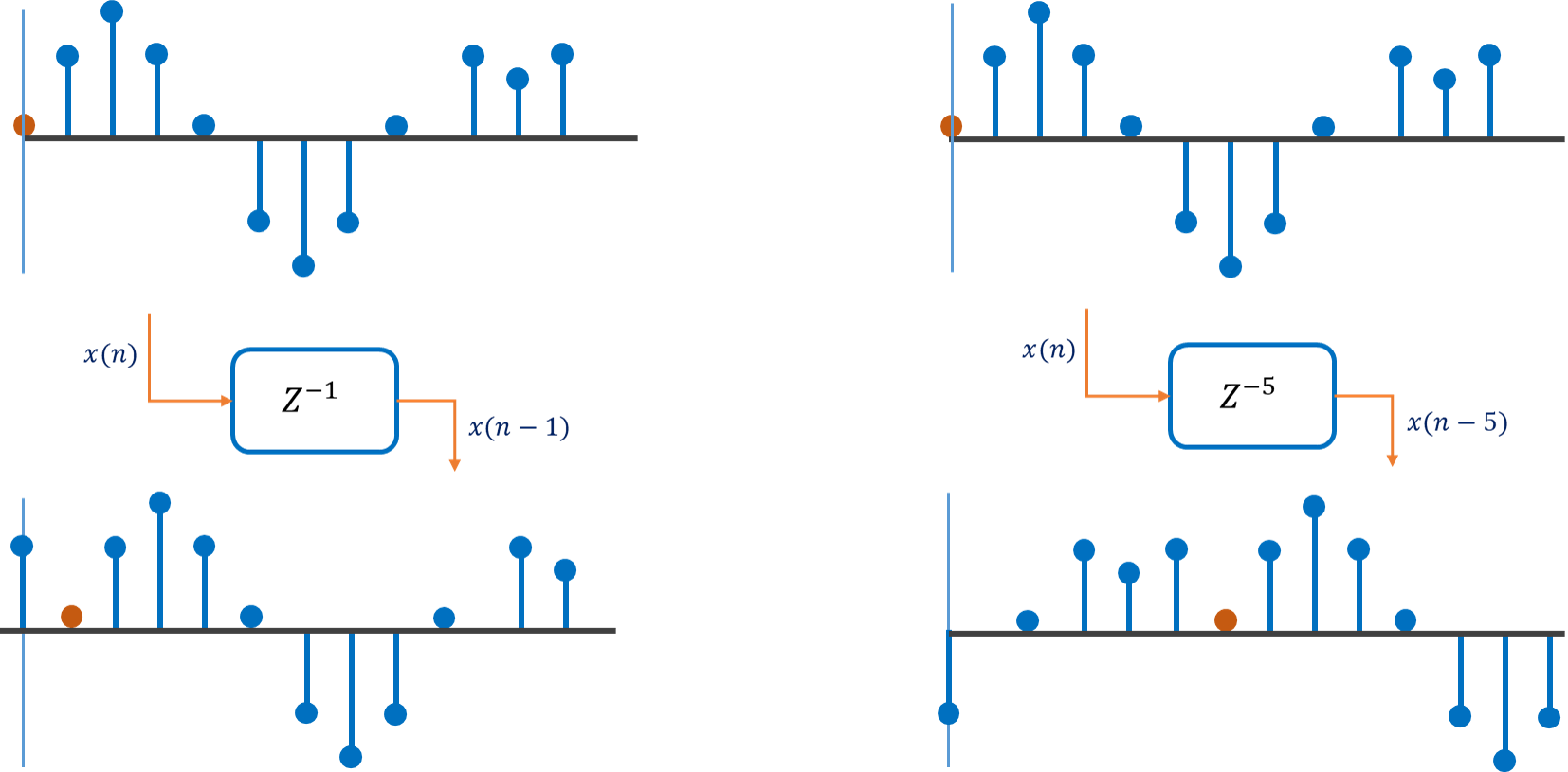
For real-time signal processing you never know what the next sample is going to be, however in non-real-time processing such as in audio files, you do know what the future samples are because they are all in the file.

Let us see the animation to understand how the delay filter works.
The key part of a digital delay is a register or a memory location when a signal passes through it. The current sample $x(n)$ is saved in the register and whatever was previously in the register is ejected and arrives at the output. This would be the previous sample $x(n−1)$. Simple at the very first bus there would not be anything in the register. So the register will simply return 0. We can cascade a number of one sample delays to get a delay block of any arbitrary number of samples. So, for example if you need a three sample delay theoretically you could just chain three separate one sample delay blocks. In essence for an N-sample delay, we would need $N$ registers or memory locations.

Example

Scalar Multiplier:

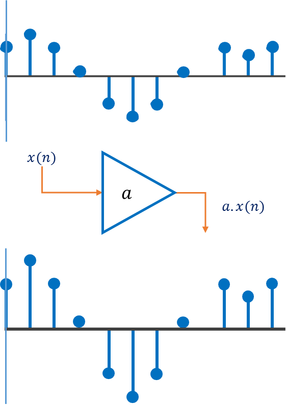
The next algorithmic building block is the scalar multiplication operation. It is a sample by sample operator that simply multiplies the input samples by a coefficient. The multiplication operator is used in just about every DSP algorithm. The symbol for scalar multiplication is a triangle which in Electronics is an amplifier. In fact the multiplication operation can be thought of as amplification. The outputs are simply scaled versions of the inputs. Notationally, if an input signal $x(n)$ passes through a multiplier block with a coefficient of a the scaled output signal would be $a.x(n)$. Figure below explains the multiplier operator.

Adder:

Finally, we have the adder block for adding or subtracting two signals. Addition and subtraction are really the same operation because subtraction is the addition of a negative number. The operation of mixing signals is really the mathematical operation of addition. The notation that is used is a circle with a sigma symbol in it. So if two signals $p(n)$ and $q(n)$ were to be combined via an adder, the resultant output would be $p(n)+q(n)$ as show in the below.

🎨 Visual Demonstration

🧠 Key Takeaways

🧠 Quick Quiz

Test your understanding of digital filters: