Feedforward Filter

🎯 Learning Objectives

By the end of this topic, you should be able to:

We will put our first foot forward into DSP in this topic with a introduction to filtering. We will use the algorithmic blocks that we saw in the topic test signals of Filter Characteristics to build a simple filter.
The most basic filter design features are in our example case:

• One delay register
• One adder
• Two scalar multipliers

The input signal passing through DSP topology will be split up into two different paths.

• A direct path to the adder, multiplied or weighted by an amplifier with a coefficient of $a_o$, and
• A delayed path through the one sample delay weighted with a coefficient of $a_1$

The two sigma-paths merge back together and the output of the circuit is the sum of the direct path and the delayed path so that would be $a_o⋅x(n)+a_1⋅x(n−1)$ because it is been delayed. This is also called the difference equation of the filter as show in the figure below.

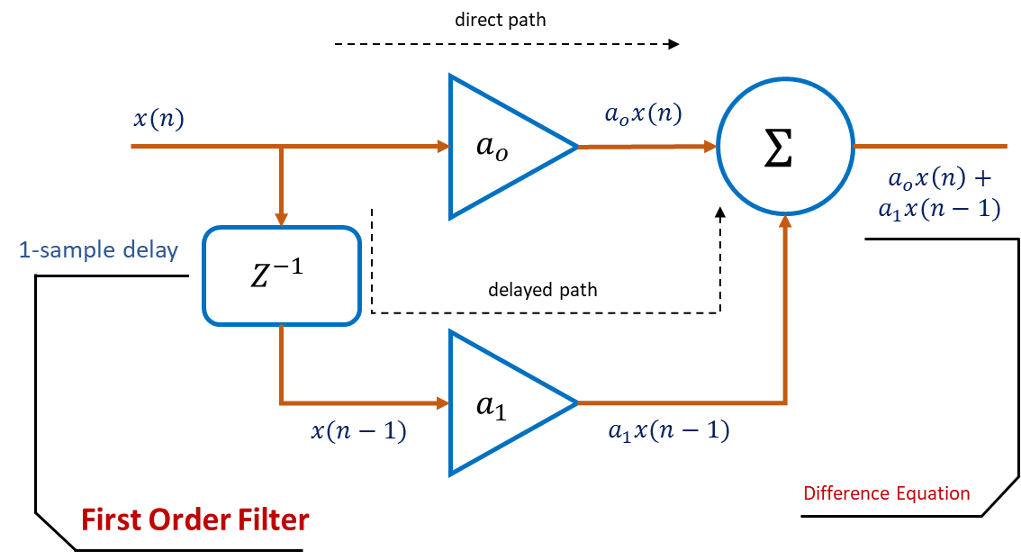
The term difference equation does not really imply any subtraction. It is just what it is called. It expresses the characteristics of the filter and gives us a relationship between the input and the output. The order of the filter is related to the number of delay elements in a signal path. There is a single one sample delay in the structure and hence it is a first order filter and we can tell why this structure is called feed forward. The input branches out feeds into the summer. The signal flows from the input to the output and there is no feedback from the output to the input which is a trait of the feedback filters that is explained in the video.

Let us assign values to the coefficients $a_o$ and $a_1$ and let us say both $a_o$ and $a_1$ are $0.5$.

What would this filter do? What are its frequency and phase responses?

In order to analyze this filter, we will take the tedious but easy approach. We discussed the topic test signals previously. The approach is to take each one of these signals and manually push the samples of the signal through the filter. One sample at a time and study the output. So we have five test signals to go through and these are:

• DC signal or the zero Hz signal
• Nyquist signal
• Half Nyquist signal
• Quarter Nyquist signal
• Impulse signal

While analyzing the filter response for an input signal for each audio sample that enters the structure the sample is read in and the output is formed by the addition of the direct weighted sample and the previous sample that was in the delay register. Incidentally the delay register is overwritten with the sample that was read. This process is illustrated in the animation below.

Analysis of DC signal or the zero Hz signal:

Let's start with the first signal, the DC or step signal with the help of animation.

However, as we saw in the animation, there is a one sample delay in the response causing the Leading Edge of the step input to be smeared out by one sample. This is called time smearing and as a normal consequence of filtering as shown in the Figure below.

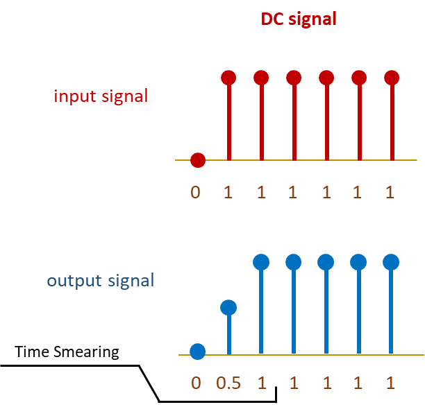
This gives us the first rule of feed forward filters:

Analysis of Nyquist signal:

Now we will repeat the process for the Nyquist frequency signal. The signal basically has two sample points for each period as shown in the Figure.

The filter behaves in an entirely different way when processing the Nyquist frequency. But we can spot the pattern after only a few iterations. So let the animation take over here.

We can see that the output completely disappears after the first sample period. The phase is kind of hard to characterize because the signal has vanished as we can see in the Figure below.

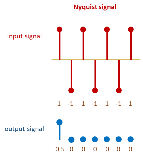
Why did the amplitude drop all the way to zero at Nyquist? The answer is one of the keys to understanding digital filter theory. The one sample delay introduced exactly 180 degree phase shift at the Nyquist frequency and caused it to cancel out when recombined with the input branch.

This leads us to the next rule:

In the case of the Nyquist signal the one sample delay is exactly enough to cancel out the original signal. When they are both added together in equal ratios. But what about other frequencies? Let us look at the half Nyquist signal to get the answer!

Analysis of Half-Nyquist signal:

Here is the output for the half Nyquist frequency signal.

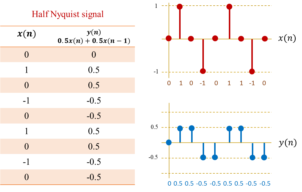
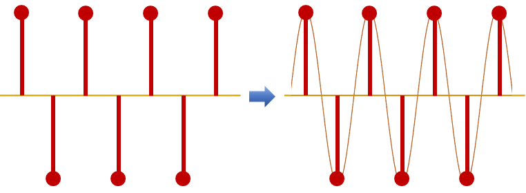
The half Nyquist signal basically has four sample points per period and the output unlike the output of the Nyquist signal has a repeating pattern though. The peak sample value registered is +0.5 on the positive axis and a −0.5 on the negative axis. If you try to inscribe a sinusoid through it and we get something like as show in the Figure below.

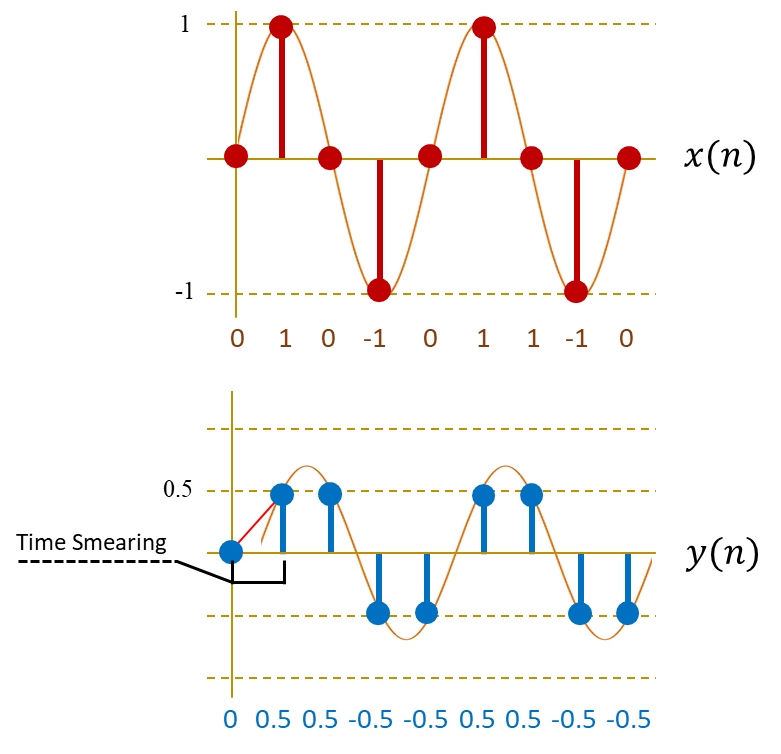
The peak of the sinusoid is around 0.7. We can notice that at the very start the output is not a perfect sinusoid. It is been dragged and stretched through time. This is basically the time smearing artifact of the filter that we discussed earlier.
So what happened here? How did we get to this output? Well, the phase shifting!
For the half Nuquist with signal the one sample delay created a 90 degree phase shifted signal unlike the Nyquist frequency which was 180 degree phase shifted and completely canceled each other out. This signal is only partially phase shifted and hence will produce an output.

Analysis of Quater Nyquist signal:

Our input signal is a quarter Nyquist frequency signal. The signal is eight sample values per period and when it is passed through the filter we get the output as shown.

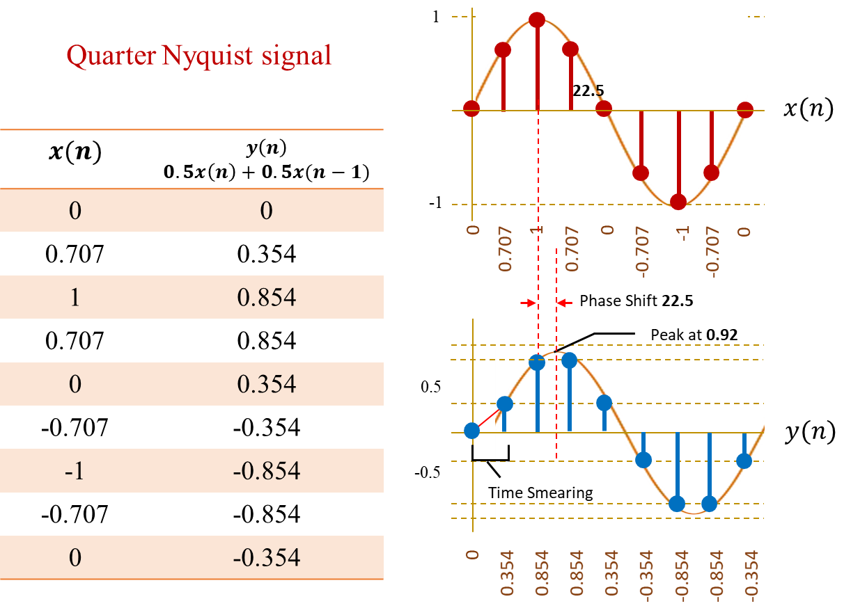
Since the quarter Nyquist signal has eight sample points the one sample delay will cause a phase shift of 1/8 which is 45 degrees of shift.
So lets see our graphing calculator again and see what the sum of the direct signal at a 45 degree phase shifted signal would look like.

Frequency Response:

Let us start with a frequency response plot with frequency on the x-axis and output amplitude on the y-axis, and let us plot the output amplitudes of each of the signals that we observed as follows.

• The 0 Hz (DC) signal was untouched by the filter so the amplitude of the output remains the same as that of the input. So it is 1.
• The Nyquist signal vanished at Nyquist frequency so we can mark its amplitude as 0.
• For half Nyquist signal, at half Nyquist frequency, we observe the peak level of the output sinusoid was 0.707. Let us mark on the plot.
• Finally, for quarter Nyquist signal, at the quarter Nyquist frequency, the amplitude was around 0.92. Let us also mark it on plot.

Figure illustrates the above steps.

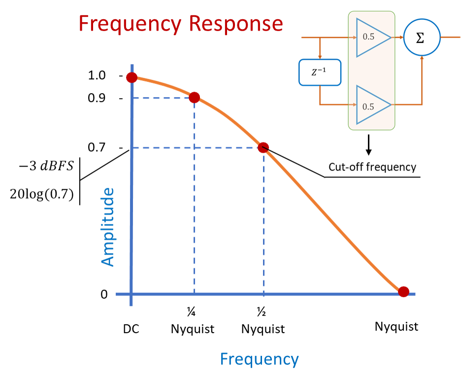
Now if we smoothly interpolate between these points, we get the frequency response of what looks like a low pass filter. In fact this feed forward filter topology that we built with its coefficients as0.5 and 0.5 is a low pass filter. It let us the lower frequencies through, unchanged, while attenuating higher frequencies. At the half Nyquist frequency the signal level is 0.707 on the linear scale, but on the logarithmic scale it is $20log(0.707)$, which is −3dB. So the cutoff frequency of this filter is fixed at half the Nyquist frequency. The cutoff frequency is solely determined by the coefficients that we have used, $a_o$ and $a_1$.
Changing these coefficients will remarkably change the frequency response of the filter.

Phase Response:

Let have a quick look at the phase response of the filter. The phase response is a straight line with no phase shift at zero degrees to a 90 degree phase shift at the Nyquist frequency. This is called a linear phase response and is not a very common thing to see in filtering. In fact this simple filter design is a linear phase filter but only under certain conditions.

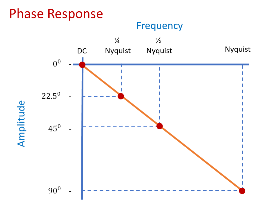
Remarks: A feed forward filter will always be a linear phase filter if its coefficients are symmetrical about their center.

In our case the coefficients that we have chosen for $a_o$ and $a_1$ are $0.5$ both and these are symmetrical. Another example would be $−0.25$ and and $+0.25$

Linear phase filters are interesting for two reasons:

• First they preserve the time domain shape of the input signal in the output. This kind of response cannot be obtained from analog filters or in IIR filters.
• Second this kind of filter has useful applications where phase linearity across the spectrum is important such as, filters for a loudspeaker crossovers or in multi-band effect processors.

🎨 Interactive Test Signal & Filter Demo

🧠 Key Takeaways

🧠 Quick Quiz

Test your understanding of feedforward filters: