Reflection of Plane Waves
🎯 Learning Objectives
By the end of this topic, you should be able to:
- Explain and apply Snell’s Law to acoustic wave reflection.
- Derive and manipulate the reflection factor for oblique incidence.
- Understand the role of specific acoustic impedance and boundary conditions.
- Compute the absorption coefficient for locally and non-locally reacting surfaces.
- Analyze limiting cases such as hard, soft, and matched boundaries.
- Model plane-wave fields using complex notation and boundary interactions.
- Apply these results to wall materials, absorbers, underwater surfaces, and architectural acoustics.
Introduction:
A plane acoustic wave interacting with a boundary such as a wall, floor, or interface exhibits reflection, transmission, and sometimes absorption depending on the boundary’s
acoustic impedance. This interaction is fundamental in architectural acoustics, noise control, underwater acoustics, and transducer design.
When a plane wave strikes a large, smooth, flat surface, the reflection is specular, meaning that
The angle of incidence equals the angle of reflection - Snell’s Law.
For an incident plane wave approaching at an angle , the amplitude and phase of the reflected wave depend on the boundary’s surface impedance.
Geometry of Incidence and Reflection
The angles of the incident and reflected waves satisfy:
Figure 1. Free-field propagation from elementary sources in direction of maximum sound radiation
The reflected wave may experience a change in amplitude and a phase shift due to interactions at the boundary.
Mathematical Description of Incident and Reflected Plane Waves:
Incident Wave
A monochromatic plane wave incident on a boundary is expressed as
where:
- is the complex amplitude,
- is the wavenumber,
- is the angle of incidence.
Reflected Wave
The reflection factor for a plane wave at oblique incidence is given by
with denoting the reflection factor,
It is related to the wall impedance, , by
where:
- is the characteristic impedance of air,
- is the surface impedance,
- is the angle of incidence.
The wall impedance, , is defined as the ratio of sound pressure to the normal component of particle velocity, both determined at the wall.c The impedance may be independent of the angle of incidence This phenomenon is called a local reaction. Due to this local reaction adjacent sections of the same wall surface are independent from each other, so that no tangential waves are transmitted along the wall surface. This is a good approximation for heavy walls, for walls with low bending stiffness and for porous absorbers with high flow resistivity.
Example:
Figure 1. Free-field propagation from elementary sources in direction of maximum sound radiation
Python Example: Plane Wave (Oblique Incidence)
2-D visualization of a plane wavefront
Press Run Code: Output will appear here.
Python Example: Reflection From an Impedance Boundary
Press Run Code: Output will appear here.
Absorption Coefficient
The absorption coefficient describes the fraction of incident acoustic energy not returned as reflection:
This is crucial in architectural acoustics and noise control.
Specific Impedance and the Reflection Fact
The specific normalized impedance is:
For locally reacting surfaces, absorption becomes:
This formulation captures complex impedance surfaces including membranes, porous layers, and micro-perforated materials.
Examples of Wall Impedances
We can define some extreme cases for perpendicular incidence. Real materials approximate these conditions quite well.
A heavy concrete wall, for instance, represents a hard wall and the ocean surface represents a soft wall for underwater sound.
Some other examples are listed as follows
- Matched wall: ; ;
- Hard wall: ; ;
- Soft wall: ; ;
Evanescent and Inhomogeneous Waves Near Boundaries:
When the angle of incidence approaches grazing incidence , the component of the acoustic wavenumber normal to the boundary becomes:
As , the normal wavenumber tends to zero, and beyond this limit becomes purely imaginary.
This yields an evanescent wave, whose pressure field decays exponentially away from the boundary:
Evanescent waves:
- Do not transport energy away from the surface,
- Can store reactive (non-radiative) energy,
- Strongly influence near-boundary pressure enhancement,
- Become significant in micro-perforated absorbers, membrane resonators, and soft surfaces.
In architectural acoustics, they contribute to surface impedance behavior and can modify the effective absorption at extreme incidence angles.
Non-Locally Reacting Surfaces and Surface Wave Propagation:
The assumption of local reaction (impedance independent of incidence angle) fails for:
- Panels with finite bending stiffness,
- Multi-layer constructions (e.g., drywall + air cavity),
- Porous materials with low flow resistivity,
- Viscoelastic or tensioned membranes.
In such cases, the boundary supports tangential (lateral) wave motion, and the impedance becomes angle-dependent:
This leads to:
- Structural–acoustic coupling,
- Surface-guided waves,
- Modal conversion between acoustic and structural modes,
- Frequency-dependent scattering.
A classical example is a thin elastic plate, where bending waves propagate with dispersion:
Here, is flexural rigidity, surface density, and bending wavenumber.
Such surfaces no longer satisfy simple reflection formulas and require solving coupled boundary-value problems.
Energy Conservation and Complex Reflection Coefficients:
For general boundaries, the reflection coefficient is complex:
It carries:
- Magnitude → how much energy is returned,
- Phase → time shift upon reflection.
The conservation law reads:
where:
- is absorbed energy,
- is reflected energy,
- is transmitted energy (zero for infinitely massive walls).
The phase contains important information:
- Soft walls exhibit a phase inversion near
- Hard walls approximate zero phase shift
- Reactive surfaces produce frequency-dependent phase changes, affecting standing wave patterns and room response.
Pressure–Velocity Boundary Layer Effects:
Very close to the boundary (within a few millimeters), viscosity and thermal conduction create a boundary layer where:
- Particle velocity is reduced due to shear,
- Pressure remains nearly unchanged,
- Local impedance deviates from its ideal value,
- Additional losses occur, especially at high frequencies.
The effective acoustic impedance becomes:
These corrections are essential for:
- Micro-perforated panels,
- High-frequency absorbers,
- Precision impedance tube measurements.
Surface Impedance of Porous Materials: Delany–Bazley–Miki Models:
Porous materials used in acoustic treatment possess complex, frequency-dependent impedance.
A classical empirical model is:
where:
- is flow resistivity,
- are empirical constants.
The impedance becomes highly angle-dependent, making the simple reflection factor insufficient.
These models are essential in room acoustics and absorber design.
Complex Pressure Fields and Standing Waves:
The superposition of incident and reflected waves yields:
This produces a standing wave ratio (SWR):
Even small reflection magnitudes () can significantly modify the pressure distribution inside rooms and ducts.
This explains:
- Bass buildup in corners (high reflection + room modes),
- Nulls at listening positions (destructive interference),
- Sensitivity in impedance measurement setups.
Plane Waves vs. Spherical Waves at Finite Distances
The plane-wave reflection theory assumes far-field incidence.
For sources close to the wall:
- Waves have spherical curvature,
- Incidence is not uniform across the surface,
- Near-field terms become significant.
The reflection coefficient becomes position-dependent:
This is important in:
- Loudspeaker-wall interactions,
- Source-to-boundary distance effects,
- Near-field microphone calibration.
Impedance of Multi-Layer Surfaces (Transfer-Matrix Method):
Real-world walls often consist of multiple layers.
Their combined impedance is computed using the transfer-matrix method (TMM):
where is the product of layer matrices.
This method captures:
- Resonances (e.g., mass–spring–mass systems),
- Phase changes through layers,
- Frequency-dependent transmission loss.
Such models are essential for wall design, studio isolation, and underwater sonar applications.
Reflection from Curved Surfaces:
For curved boundaries, Snell’s law applies locally, but curvature introduces:
- Focusing or defocusing of reflected rays,
- Spatially varying reflection coefficients,
- Modified standing wave fields,
- Potential caustics (regions of high intensity).
This becomes important in:
- Whispering galleries,
- Curved auditorium walls,
- Reflective domes and parabolic surfaces.
Numerical Approaches to Plane-Wave Reflection:
In complex geometries, analytical solutions fail.
Numerical methods used include:
- Boundary Element Method (BEM),
- Finite Element Method (FEM),
- Transfer-Matrix Method (TMM),
- Ray-tracing with frequency-dependent reflection,
- Parabolic Equation (PE) models (underwater acoustics).
These methods allow modeling:
- Arbitrary surface geometry,
- Frequency-dependent impedance,
- Complex scattering scenarios.
Spherical Wave Above Impedance Plane:
A point source at radiates a spherical wave. The total field at contains a contribution from the direct sound travelling along the vector and another component reflected from the plane.
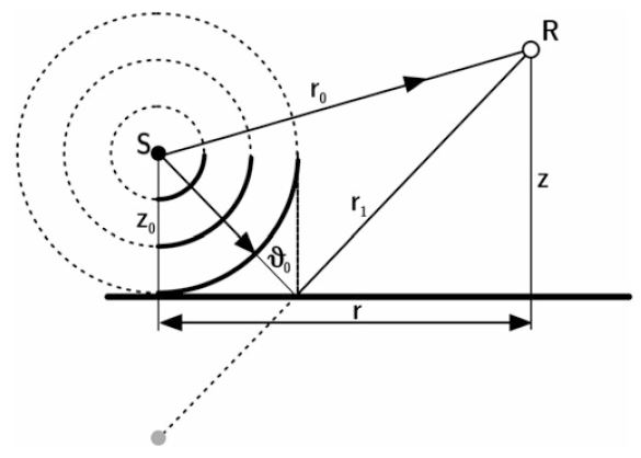
Figure 1. Spherical wave reflection above impedance plane
A plane wave incidence and a spherical wave incidence differ significantly as the impedance plane is hit at various angles and the total reflection must be integrated:
The first term represents the direct sound and the latter the contribution of the reflection.
Note that the reflection term is an integral over various angles between the wavefront and the surface.
An approximation of the entire expression assuming a constant angle of incidence, , is
This equation assumes a constant angle and, thus, a plane wave.
Now, the contribution of the reflection can be related to another point source, called the image source, which is apparently located
below the surface radiating a spherical wave whose amplitude is reduced by .
Even though a spherical wave is present, the reflection is calculated for a constant angle . The sound field model is effectively switched to a plane-wave description when reflection occurs. This image source model is even accurate when or . For other reflection factors, the approximation is sufficiently accurate when , , and .
In a reflecting plane, plane waves or spherical waves can be divided into elementary sources (Huygens principle). Together these sources build up an interference field that produces a plane or spherical wave. This model is the basis for the simplicity of Eq. (which is exact when ).
If, however, the plane has discontinuities in geometry or impedance, the Huygens superposition is disturbed and the reflected field exhibits scattering and diffraction. Scattering results from reflection by an object; diffraction results from interaction with the edges or boundaries of an object.
🧪 Interactive Examples
📝 Key Takeaways
- Plane-wave reflection is governed by Snell’s law, ensuring that the angle of incidence equals the angle of reflection for smooth, large surfaces.
- The reflection factor depends on the surface impedance and incidence angle and determines both the amplitude and phase of the reflected wave.
- Surface impedance encapsulates the mechanical and acoustic behavior of the boundary and can be real (resistive), imaginary (reactive), or complex.
- The absorption coefficient quantifies the fraction of acoustic energy not returned as reflection and depends strongly on the impedance and angle of incidence.
- Locally reacting surfaces have angle-independent impedance, while non-locally reacting surfaces support tangential wave motion and require structural–acoustic models.
- Evanescent waves arise near grazing incidence and influence near-boundary pressure fields without transporting energy away from the surface.
- Hard, soft, and matched boundaries represent important limiting cases and guide practical design in architectural, underwater, and engineering acoustics.
- Advanced models such as Delany–Bazley, transfer-matrix methods, and complex impedance formulations provide realistic predictions for layered or porous materials.
🧠 Quick Quiz
1) What determines the phase shift experienced by a reflected plane wave?
2) For a matched boundary where , what is the reflection coefficient ?
3) What is the defining characteristic of a locally reacting surface?
4) Which phenomenon occurs when the normal component of the wavenumber becomes purely imaginary?
5) The absorption coefficient is given by . What does this physically represent?